Jupyter Notebook Db2 Client
Dean Compher
29 March 2019
There is a new Db2 client you may want to consider for your desktop. It is the free Jupyter Notebook. I recommend trying it out even if you already use a client like the CLI, Data Studio, Toad or something else. Like other clients, you can define your connections, and just click on the one you want when you query the database. I like it for a number of reasons including the way it displays the results, allows some very easy graphing, easy query sharing, its lightweight and allows you to easily create scripts to process data that you return from your queries. While it is new to me, I like Python for scripting. It is easy to use, and I now impress my friends and colleagues by talking about programming in Python.
In this article I’ll show some of the things that I like about using the Jupyter Notebook as a Db2 client, and then provide links for installing it. There is is a great facility where you can get a hands-on trial to quickly learn the basics of notebooks and Db2 on the IBM cloud, so you can decide if it is worth installing on your workstation. I’ve put that link for that below as well as the links for where you can get the Jupyter Notebooks and the Db2 extensions for the notebook.
Here is a sample of what I have at the top of all of my notebooks:
Example 1. Database Connections
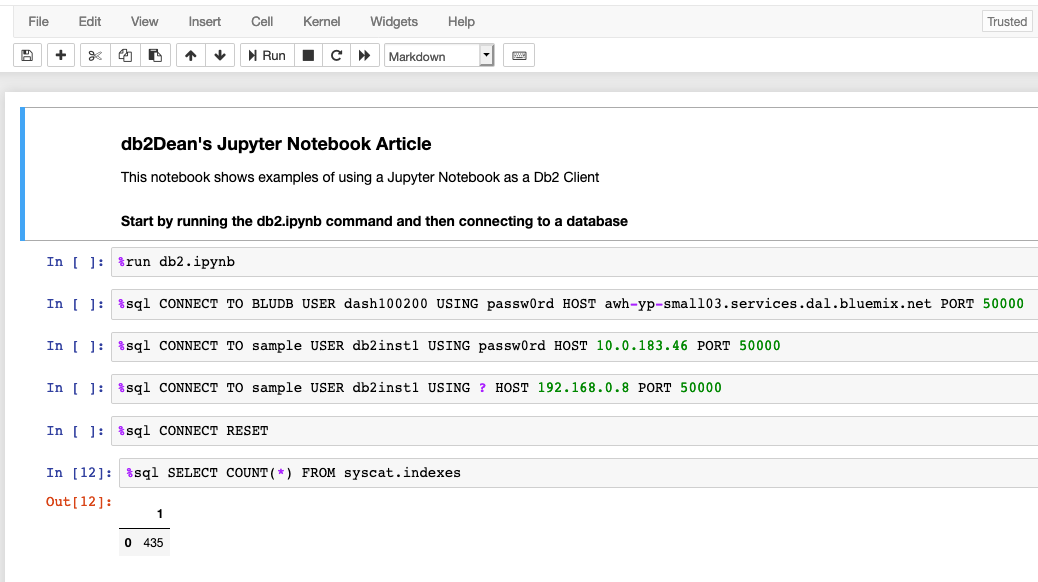
When I want to query my database, I open up my notebook, run the first cell that runs the db2.ipynb notebook and then I connect to the database that I want to use by executing the cell with the connect command for that data base. I then run the last cell shown where I count the number of indexes just to make sure that I’m really connected. When I want to query a different database, I just scroll back to the top of my notebook, run the CONNECT RESET cell, and then run the cell that connects me with my desired database. You do not need to code your password. You can instead place a question mark as shown in the third connect example above and you will be prompted for the password.
When I say “cell” I mean one of the gray boxes with the commands. These are called “code” cells and you can enter code into them. Notice that all of these commands started with the “%sql” command. This is what allows you to connect to- and query- the database without writing a lot of python code. This functionality is made available by running the first cell with the ”%run db2.ipynb” command. Commands starting with the percent sign are called “magic” commands.
The other type of cell that you will commonly use is the is called a “markdown” cell and there is where you add comments and documentation. The first cell in this example is a markdown cell and starts with “db2Dean’s Jupyter Notebook Article”. It is pretty easy to format the comments. You can insert, delete, copy and move cells around as you like. How to format text in the markdown cells is covered early on in the trial that I will discuss later.
Example 2. Query Db2, display results and use input variables
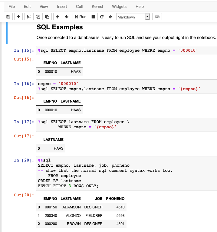
In the example above I show 4 examples of querying the database and the output. In the first three I use the %sql syntax that allows you to have one line of query unless you use the continuation mark (back slash) as shown in the third example. In the last line I use the %%sql command that allows you to code the query over multiple lines without a continuation. Unfortunately, the %%sql command does not allow you to use variables like you see in the second and third examples. Also notice in the third example I used the “empno” variable but didn’t define it there. That’s because I first ran the previous cell where it was defined, and the definition persists through any subsequently run commands.
You cannot use variable substitution with the CELL version of the %%sql command. If your SQL statement
extends beyond one line, and you want to use variable substitution, you can use
a couple of techniques to make it look like one line. The simplest way is to
add the backslash character (\) at the end of every line. Example 3
illustrates the technique.
In addition to being able to define variables that you use in your SQL, you can also grab values out of the database to be used in your scripts. Using the %sql Db2 Magic commands you can assign the output of a query to a variable. The output will be a matrix of rows and columns. Here is an example of using the output of a query to generate RUNSTATS commands using Python code. Notice in the last cell where I both run the RUNSTATS command using the %sql magic command and display the RUNSTAS command using the print function.
Example 3. Load query results into Python variable and use it in scripting
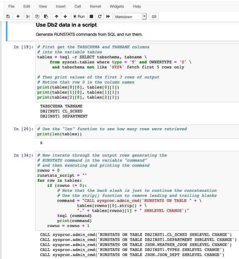
This is a rather basic use of the data extracted from the database, but it serves the purpose of showing how to get data from a table and use it in a script. Once you have the data in a variable (in this case the variable name is “table”), there is no limit to what you can do with it in your notebook. You could do any number of advanced statistical functions on it, use it to train data models, our use Python’s and Jupyter’s graphing capabilities. In this case I just generated runstats commands and executed them on the database through the Db2 admin_cmd built-in stored procedure using the %sql magic command.
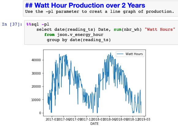
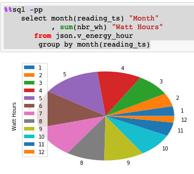
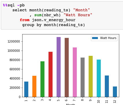
Another really useful thing you can do is to perform simple graphing of any two columns you can select from your database. While the level of graphing is limited, it is extremely easy to use. You can create line, bar and pie charts using a select of any two columns in the database. You just indicate the correct option after the %sql command and instead of showing the text, they are graphed for you. In the following examples, I use data from the solar system on my home that I have been collecting for about two years now. In the first chart you can see the cyclical nature of production by using the -pl parameter to produce a line chart from the query output.
Example 4. Graphs of queried data
Here are examples of using the same v_energy_hour database view to show total production for by month of the year (1=Jan, 12=Dec) using both a pie chart (-pp) and a bar chart (-pb). Python doesn’t care if you reference tables orviews. Again, you can see that the more energy gets produced in the summer months. If you are an avid follower of db2Dean.com, then you may recognize that the json.v_energy_hour is similar to the view on a JSON document I created in last month’s article.
Notebooks are saved to files. So once you create a notebook with all of your connections and some interesting SQL, you can just e-mail it to a colleague and they can work with what you have done. When doing this you will probably want to substitute real passwords with the “?” prompt. Since we are discussing sharing, I have posted the notebook I created for this article on the website and you are welcome do download it.
Try it for yourself for free in the cloud
George Baklarz and his team have created an amazing tutorial for learning how to use Jupyter Notebooks and Python with Db2. You can get your hands on this tutorial at this link on the IBM Digital Technical Experience site.
The tutorial gives you a VM with Db2 and Jupyter up and ready to go. This lab actually shows you how to use more than those two use cases, so if you are only interested in those topics then you can just do Labs 2, 3 and 4. You may need to do some of Lab 1 to get the credentials for the Db2 database. These labs give you much more information on how to use Jupyter and Python with Db2 and are a great way to get started.
Installing Python, Jupyter and the Db2 Magic commands
Once you have taken the test drive and have decided that the Jupyter Notebook client for DB2 is for you, then it is time to install it using these instructions are on Git Hub in the Juypter Db2 Samples directory.
Start by reading the “installation.md” instructions near the bottom of the list.
1. Note that that instructions indicate that you get Python from www.continuum.io That site no longer works. Now you down load it from anaconda.com site.
2. This document provides instructions for Linux and Windows. To install the Db2 add-ons to your new Python environment on Mac, use the Linux instructions with the following additions and exceptions:
a. Run the two “conda” commands as shown in the instructions from a terminal window.
b. The apt-get and easy_install commands did not work for me. Instead I did the following:
c. Installed Homebrew. Since you now have Python, install the following commands should work from a terminal window:
$ brew install -y gcc
d. Next add the db2 components to python from the terminal window:
$ easy_install ibm-db
Next go back to the db2jupyter directory and download the db2.ipynb file. Notice the green “Clone or download” button in the upper right of this page. Execute this notebook as the first step in your notebooks accessing Db2 to get the Db2 magic commands. Read the README.md instructions in the db2jupyter directory to see how to use the file and some examples of using the notebook.
There are also several additional notebooks in this directory with examples of lots of good things you can do. If you discover any creative uses for Jupyter notebooks for Db2 please post them on my Facebook Page or my db2Dean and Friends Community along with any other comments you may have.